Hands-on Spectral Normalization
A brief explanation and some code snippets related to spectral normalization


Spectral normalization is a widely used technique to stabilize and improve the training of Generative adversarial networks. In nutshell, this normalization technique allows the measurement of meaningful distance between real and generated examples using discriminator. This measure is then used to train both, the discriminator and the generator.
In my previous post I have walked through changes proposed in WGAN paper skipping an import piece about Lipschitz constraint. In this post I will discuss the most effective (up to this day) technique to satisfy this constraint.
As we talked in previous post, work of the authors of WGAN paper proposed to use the distance between the outputs of the discriminator as a proxy for distances between distributions. To put it simply, we want to measure how far two distributions are from each other. In order to be able to use the discriminator output as a proxy, we need to bound discriminator to be Lipschitz constrained.
Spectral Normalization
Interestingly, the authors of WGAN paper turned to the AI scientific community for the best approach. And a year later the paper called Spectral Normalization for Generative Adversarial Networks came out with a proposed solution. In comparison to previous attempts, this solution was superior due to its efficiency. So let's dig into it.
According to the paper, the Lipschitz constraint of the layer can be satisfied by dividing the weights of the layer by the largest singular value of the same weights. A really nice explanation and proof can be found here. Mathematically it looks like this:
$$W=W/\sigma(W)$$
where $\sigma(W)$ is the largest singular value of the weights $W$.
An important observation by the authors of the paper is that if we do it for all layers, we will have a network that satisfies Lipschitz constraint.
Sounds simple enough, let's try it out.
import numpy as np
Let's take a convolutional filter of kernel size 3x3, 256 input channels and 512 output channels. Note: we reshaped the kernel so that we could calculate singular values.
W = np.random.normal(size = [3,3, 256, 512]).reshape([-1,512])
W.shape
Let's use numpy library to find singular values. numpy.linalg.svd can do that for us. The second output of numpy.linalg.svd function returns all singular values, we just need a maximum of that.
%%timeit
s = np.linalg.svd(W, full_matrices=True)[1].max()
s
That is quite simple, however, it takes 1 second to calculate those values. Let's assume that we have 30 layers in the network, that would mean extra 30 seconds for each training step. Well, that is not what we could call efficient.
from scipy.sparse.linalg import svds
There is an alternative. scipy.sparse.linalg.svds function returns only the number k of the largest singular values.
%%timeit
s = svds(W, k=1)[1]
s
This is much faster: ~74ms, however for 30 layers we will slow down the training process by 2 seconds per step. Still not ideal.
Luckly, The authors of the paper proposed an alternative solution to get the largest singular value. This technique is known as power iteration. This looks like this: $$ v = W^\intercal u / ||W^\intercal u||_2$$
$$ u = W v / ||W v||_2$$
$$ W = W / u^\intercal W v$$
Let's see if we can implement it.
$u$ needs to be sampled from an isotropic distribution at the beginning and it's dimensions should match the dimensions of the number of output channels.
u = np.random.normal(scale=0.2, size=[512])
u.shape
First row of the equation
Note: we swapped u and W just for the sake of simplicity when implementing in numpy
v = u@W.T/np.linalg.norm(u@W.T, 2)
v.shape
Second row of the equation
u = v@W / np.linalg.norm(v@W, 2)
u.shape
Third row of the equation
sigma = v@W@u.T
sigma
Let's put everything together
def get_largets_singular_value(u):
  v = u@W.T/np.linalg.norm(u@W.T, 2)
  u = v@W / np.linalg.norm(v@W, 2)
  sigma = v@W@u.T
  return sigma, u
%%timeit
sigma, _  = get_largets_singular_value(u.copy())
print("Answer from numpy:", svds(W, k=1)[1].squeeze())
print("Power iteration outcome", sigma)
Well, it is fast, ~40x faster, but it is not accurate. Well, that is expected because power iteration only approximates the largest singular value. The more iterations you perform, the more accurate approximation you would get.
Let’s see if that is true.
u_copy = u.copy()
actual = svds(W, k=1)[1].squeeze()
for i in range(20):
  sigma,u_copy = get_largets_singular_value(u_copy)
  print("Power iteration estimate: {:.2f} (actual: {:.2f})".format(sigma, actual))
This is indeed the case. However, doing power iteration 20 times gets us close to scipy performance. Fortunately, Spectral Normalization paper showed that you can do one or a small number of iterations per training step to get a good estimate throughout the entire training (doing incremental work every step). Hence, even using naive numpy implementation we can get to only extra 60ms (1.7ms*30) for each training iteration (assuming 30 layer network).
That does not sound too bad.
Note: keep in mind that these performance numbers are relative, they will depend on hardware.
We can try to port this to tensorflow and measure its performance.
import tensorflow as tf
tf.config.list_physical_devices('GPU')
@tf.function
def get_largets_singular_value_tf(u, w):
  _v = tf.matmul(u, w, transpose_b=True)
  _v = tf.math.l2_normalize(_v)
  _u_m = tf.matmul(_v, w)
  _u = tf.math.l2_normalize(_u_m)
  sigma = tf.matmul(_u_m, _u, transpose_b=True)
  return sigma, _u
u_tf = tf.Variable(tf.random.normal(stddev=0.2, shape=[1,512]), trainable=False)
w_tf = tf.Variable(tf.random.normal(shape = [3*3*256, 512]), trainable=False)
%%timeit
sigma_tf, _ = get_largets_singular_value_tf(u_tf, w_tf)
for i in range(20):
  sigma_tf, u_tf = get_largets_singular_value_tf(u_tf, w_tf)
print(sigma_tf)
That is even better. 509µs with tensorflow implementation and executed on GPU (which usually is the case when you are training GANs). So if we assume 30 layers of similar size and one power iteration per training step, we only need ~15ms extra for the step. That is the reason why this technique is widely and successfully adopted.
Since we have all the pieces, we can create a layer wrapper to wrap any layer and perform power iteration on each feed forward pass. I have extended the code of here I have incorporated suggestions from the comments:
- Turned off power iterations during the inherence. This makes sure that weights are not being changed doing inherence.
- Used assigned operation instead of
=. This speeds up the algorithm quite significantly (roughly by 35%).
Additionally I have also added a hack to support mixed precision as well as the logic to support embedding layers. The final solution looks like this:
class SpectralNormalizationV2(tf.keras.layers.Wrapper):
    """
    Attributes:
       layer: tensorflow keras layers (with kernel or embedding attribute)
    """

    def __init__(self, layer, eps=1e-12, **kwargs):
        super(SpectralNormalizationV2, self).__init__(layer, name=layer.name + "_sn", **kwargs)
        self.eps = eps
        self.is_embedding = isinstance(self.layer, tf.keras.layers.Embedding)

    def get_kernel_variable(self, attr='kernel'):
        if not hasattr(self.layer, attr):
            raise ValueError('`SpectralNormalization` must wrap a layer that contains a `{}` for weights'.format(attr))
        return getattr(self.layer, attr)


    def build(self, input_shape=None):
        if not self.built:
            super(SpectralNormalizationV2, self).build(input_shape)
            if self.is_embedding:
                self.w = self.get_kernel_variable("embeddings")
            else:
                self.w = self.get_kernel_variable()

            self.autocast = hasattr(self.w, "_variable")
            self.last_dim = self.w.shape[-1]
            self.u = self.add_weight(shape=[1, self.last_dim],
                                     initializer=tf.keras.initializers.TruncatedNormal(stddev=0.02),
                                     name='sn_u',
                                     trainable=False,
                                     experimental_autocast=False)

    @tf.function
    def call(self, inputs, training=True):
        # Recompute weights for each training forward pass
        if training:
            self._compute_weights()
        output = self.layer(inputs, training=training)
        return output

    def _compute_weights(self):
        """Generate normalized weights.
        This method will update the value of self.layer.kernel with the
        normalized value, so that the layer is ready for call().
        """
        if self.autocast:
            w = self.w._variable
        else:
            w =self.w
        w_reshaped = tf.reshape(w, [-1, self.last_dim])
        _v = tf.matmul(self.u, w_reshaped, transpose_b=True)
        _v = tf.math.l2_normalize(_v, epsilon=self.eps)
        _u_m = tf.matmul(_v, w_reshaped)
        _u = tf.math.l2_normalize(_u_m, epsilon=self.eps)
        sigma = tf.matmul(_u_m, _u, transpose_b=True)

        self.u.assign(_u)
        self.w.assign(w / sigma)

    def compute_output_shape(self, input_shape):
        return self.layer.compute_output_shape(input_shape)
And the way you use is:
dense_sn = SpectralNormalizationV2(tf.keras.layers.Dense(units=100))

conv_sn = SpectralNormalizationV2(tf.keras.layers.Conv2D(filters=256, kernel_size=3))

emb_sn = SpectralNormalizationV2(tf.keras.layers.Embedding(input_dim=20, output_dim=100))
I have also checked the performance in comparison to Pytorch implementation
Setup:
- Batch size: 64
- Kernel of size :[16, 16, 256, 512]
- Steps: 1000
- One power iteration per step
- Hardware: NVIDIA V100
Results are:
- Elapse time of Tensorflow SpectralNormalizationV2: 1.1081128120422363s
- Elapse time of Pytorch official SpectralNorm implementation: 1.0783729553222656s
Pytorch seems to be a little bit faster. I am not entirely sure whether it has to do with implementations of spectral normalization or just to the differences between Pytorch and Tensorflow. Regardless, those extra 30ms every 1000 steps should not be a game changer.
Summary
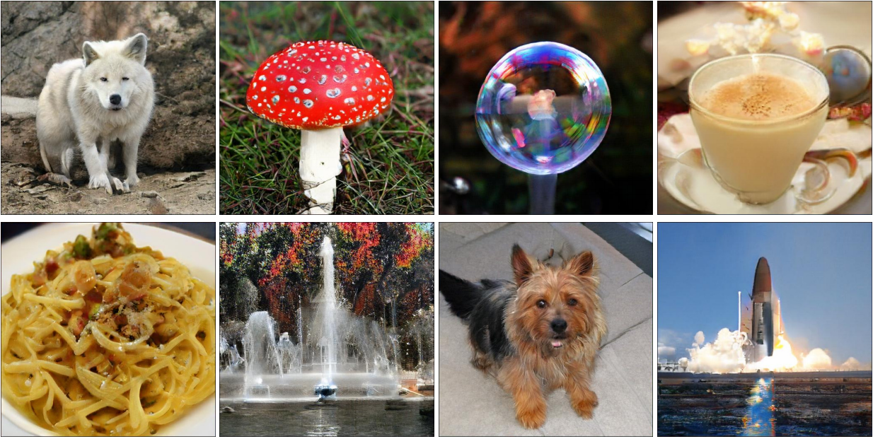
Spectral normalization is quite widely used in various implementations of GANs. One of the most famous applications is Biggan. All images below are generated by BigGAN architecture that uses Spectral normalization. This should highlight the importance of this advancement.
Throughout this post we focused on the implementation of power iteration proposed in Spectral Normalization for Generative Adversarial Networks paper. We have compared various methods to calculate the largest singular value and observed that the proposed power iteration method is the fastest and after multiple iterations it achieves reasonable accuracy.